Encoding Shapes for Machine Learning Applications
When I was an undergraduate Geography major in the 1980s, Geographic Information Systems (GIS) was a fairly new discipline. One of my courses actually used what people called "the world's first GIS textbook". People would still debate the relative merits of making maps with computers versus paper, ink, and drafting tools. For one inclined towards technology and analytics, the notion of digital mapping and geospatial analysis was, well, exciting enough to convince me to make a career of it.
A big topic in those early days of GIS was the difference between "raster" and "vector" approaches. Any software that called itself a GIS was typically either one or the other. Raster systems represented the world as data points on a grid, which includes imagery or any quantity that is known at regular intervals. Vector systems (like the original "Arc/Info", now known to the world as ArcGIS), instead represented spatial objects as geometries: points, lines, and polygons defined by strings of coordinates, to which one may assign whatever attributes are relevant for a particular application.
The differences between raster and vector systems were so significant that people would speculate that one might eventually win out, and the other would be relegated to the dustbin of outdated technology. After all, we had seen vector graphics technology (remember the Asteroids arcade game?) steadily replaced with imaging and video. Maybe something similar would happen in the GIS world.
Of course we know now that that didn't happen. Both raster and vector approaches are still with us, because each has distinct merits. For example it would be hard to represent a continuous quantity like temperature as any kind of vector object, and objects with precise positions and interrelationships like road segments lose a lot when represented as a raster.
Geospatial machine learning
Over the last decade, some of they key developments in Artificial Intelligence and Machine Learning (AI/ML) have been in the processing of images – image labeling, captioning, object recognition and so on. This emphasis on "raster" data in AI/ML shows in the way that these technologies are applied to geospatial problems. Most online material and blogs that cover Geospatial AI (GeoAI) have a strong emphasis on the use of satellite and airborne imagery. And while the community clearly recognizes the potential for vector-format geospatial data in AI/ML systems, the subject is arguably less developed than the handling of imagery and other gridded data. Which means there are still a lot of great research challenges in GeoAI with vector-format data.
One issue is that traditional machine learning models – regressors, classifiers, clustering algorithms and so on – expect their inputs to be vectors of numbers, or at least entities that can be converted into vectors using methods like one-hot encoding. Geometries, in contrast, can be represented in a number of ways, with a typical one being the Well-Known Text (WKT) format. (Of course it's really only "well-known" among people who do spatial analysis, but that's the name and we'll stick with it.) For example the WKT specification for a point looks like POINT(1 1), and a line segment might be LINESTRING(0 0, 1 1, 2 3). There is no particular limit to how big a WKT string can be; the LINESTRING defining a long river might have hundreds or thousands of coordinate pairs.
The three "primitive" types of geometries represented in WKT are the Point, LineString, and Polygon. There are also types MultiPoint, MultiLineString, and MultiPolygon for objects that are collections of the primitive types. For example an intersection of a pair or roads might be represented as a Point; the set of all traffic lights in a city might be better considered a single MultiPoint entity rather than a set of separate Point objects, depending on the application.
Vast quantities of vector-format data are available for geospatial analysis. For example data from OpenStreetMap and The Overture Maps Project are represented using those geometry types. And demographic information like the US Census American Community Survey is referenced to vector-format data representing administrative units.
Positional encodings for geospatial objects
ML models are simply not set up to ingest data represented in this way. (Unless we're talking about Large Language Models (LLMs), but that's a topic for another day.) For that reason, the field of Spatial Representation Learning (SRL) has arisen in recent years. (Mai24b). The idea of SRL is to create representations of spatial geometries that can be understood by machine learning models. In other words, we seek vectors of numbers that somehow capture the relevant geometric attributes of spatial objects. That lets us feed shapes to models.
Existing approaches to SRL were reviewed and categorized in Mai22. Their taxonomy defines an embedding $\mathbf{m}$ of a geometry $\mathbf{g}$ as a composition of two types of processing.
\[\mathbf{m} = \mathrm{NN}(\mathrm{PE}(\mathbf{g})) \]
The first operation is "positional encoding" $\mathrm{PE}(\mathbf{g})$, which is an initial conversion of the geometry $\mathbf{g}$ into some vector representation. That is, you put in a geometry and get out a vector, typically the result of some well defined algorithmic procedure.
The second operation is the use of a neural network $\mathrm{NN}$ to learn an embedding for these positional encodings. The NN takes the positional encoding and transforms it into a representation that is well adapted for input to downstream prediction and classification problems, even if it is not intuitively explainable since it comes from a black box.
Common approaches for the NN part are similar to those used for representation learning in other domains: one or more neural network layers are trained to solve a self-supervised problem, and the model's intermediate layers are assumed to yield a useful embedding for the inputs. Those embeddings can then be used for downstream ML/AI processing.
For the Positional Encoding part, a lot approaches have been proposed, and were reviewed in Mai22 and Mai24a. Many methods are specific to a particular type of geometry – either Points, LineStrings or Polygons individually – which complicates their use for general spatial analysis. In fact Mai24a specifically highlights the need for "a unified representation learning model that can seamlessly handle different spatial data formats".
The point of this blog post is to discuss steps towards such a unified approach, presenting an approach that can be applied to any type of geometry.
Multi-Point Proximity (MPP) encoding
A promising method discussed in Mai22 is "kernel-based location encoding". The technique was initially described in Yin19 under the name GPS2Vec, as a way to encode GPS coordinates at global scales. We start by defining a grid of reference points $\mathbf{r} = [r_i: i \in 1..n_r]$ covering some region. Then for a point $p$ to be encoded, compute the value of a kernel function based on the distance between $p$ and each reference point. The kernel function is a negative exponential with a scaling factor. The ordered set of kernel values is the positional encoding $\mathbf{e}(p)$ for the Point $p$:
\[\mathbf{e}(p) = \Big[ \exp\Big( \frac{-\|p-r\|}{s} \Big), r \in \mathbf{r} \Big] \]
where $\|p-r\|$ is the distance (typically Euclidean) between a reference point $r$ and the to-be-encoded point $p$, and $s$ is a scaling factor. [A not-bad choice for $s$ is to use the same value as the spacing between reference points.] Using this framework, any $(x,y)$ coordinate can be represented as vector of size $n_r$.
The original GPS2Vec aims to define a world-wide reference system. So the grid of reference points is defined relative to the Universal Transverse Mercator (UTM) system, which covers the entire world. But nothing in the design of the method limits its application to UTM zones, and one could use any coordinate system or map projection, covering regions of any extent. There is even nothing inherently "geographical" about the approach, and it could be applied in any 2D reference frame, such as a building floor plan, a circuit board design, or pixel coordinates for a digital image.
We can make a straightforward extension to the GPS2Vec approach, defining the distance $\mathrm{d}(\mathbf{g}, r)$ as the nearest-point distance from any geometry $\mathbf{g}$ to a reference point $r$. This is, in fact, the most common definition of "distance" between a pair of arbitrary geometries, and is what you get by default from widely used tools like the shapely package in python.
\[\mathbf{e}(\mathbf{g}) = \Big[ \exp\Big( \frac{-\mathrm{d}(\mathbf{g}, r)}{s} \Big), r \in \mathbf{r} \Big] \]
That is, given a set of reference points, any geometry can be encoded as a vector of size $n_r$, based on its proximity to the reference points. We can call this Multi-Point Proximity (MPP) encoding.
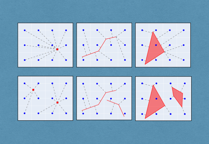
Examples of MPP encoding are shown below. We have defined a region measuring $400 \times 300$ units, and laid out a $3 \times 4$ grid of reference points spaced 100 units apart (the blue dots in the figure). Then we compute the closest-point distance between the reference points and geometries, and apppy the kernel function above, using a scaling factor of 100 units. A "flattened" representation of the kernel values gives us a 12-element encoding for each shape.
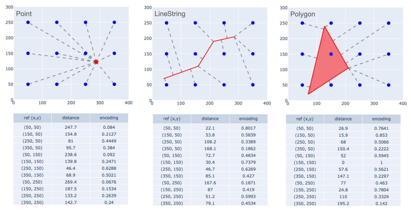
Note that for the Polygon, the reference point that lies in the interior has a distance of zero, and applying the kernel function yields a value of 1. Given the use of a negative exponential kernel, any reference point that lies in or on a shape yields a value of 1, and the value is strictly positive and monotonically decreasing with distance. So every element of an encoding lies in the interval $(0, 1]$, which is a nice range for use with neural networks.
The same procedure can be applied to "Multipart" geometries.
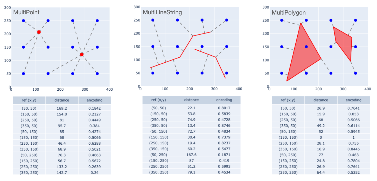
The plot on the left, for example, should not be seen as separate encodings for the two points, but as a single encoding for a 2-element MultiPoint geometry. A similar point of view should be taken for the MultiLineString and MultiPolygon examples.
Captutring geometric properties
MPP encoding lets us represent any of the 6 basic geometry types using a consistently defined and consistently sized vector. That gets us past the main hurdle to encoding shapes for ML models: coming up with a conformable representation for arbitrary geometric objects. But we still need to demonstrate that the encoding is useful. In this section I'll give a couple of examples to show that the MPP captures some important properties of the shapes that they encode.
Clustering shapes
Typically clustering algorithms are applied to point data: each data element is a point in n-dimensional vector space, and clusters are based on how close points lie to one another. Since MPP encodings are n-element vectors, they can be used in that way.
Below, the left plot shows a few line segments within a region measuring $100 \times 100$ units. We have defined a $5 \times 5$ grid of reference points spaced at 20-unit increments. So each individual line segment gets MPP-encoded as a 25-element vector.
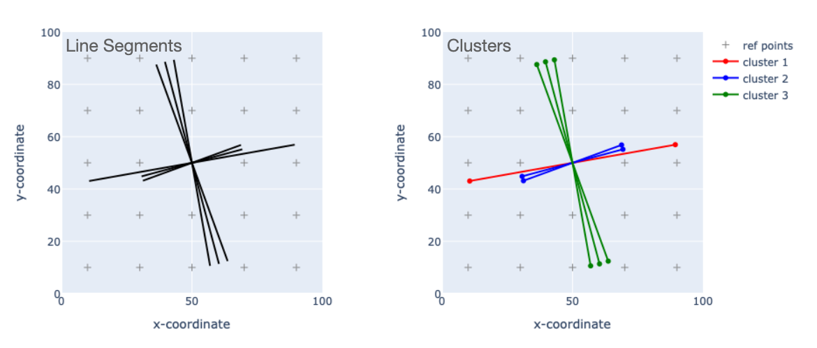
Though I'm not showing the vectors here, one can feed them to a clustering algorihtm. I used DBSCAN since it can create clusters of any size and doesn't require a lot of data to estimate distributional parameters. It can also create a "cluster" of one element when it is appropriate to do so. Using an epsilon parameter of 0.5 yields the three clusters shown on the right. DBSCAN has grouped together the three almost-vertical segments. And among the three almost-horizontal segments, we have two groups distinguished by segment length.
Although this is a trivial example, it's important to note what's happening. We started with a few geometries that all occupy the same general part of the reference frame, and in fact all have the same centroid. Then using MPP encoding, we have grouped these shapes based on similarities in orientation and length. This is good evidence that the MPP encodings characterize spatial similarities and differences.
Here is another example. The plot on the left shows a pair of LineStrings crossing a $100 \times 100$ region. There are also two MultiPoint objects. While there is a lot of scatter to the ponts, one can see that the green diamonds roughly follow the orange line while the red circles follow the blue one.
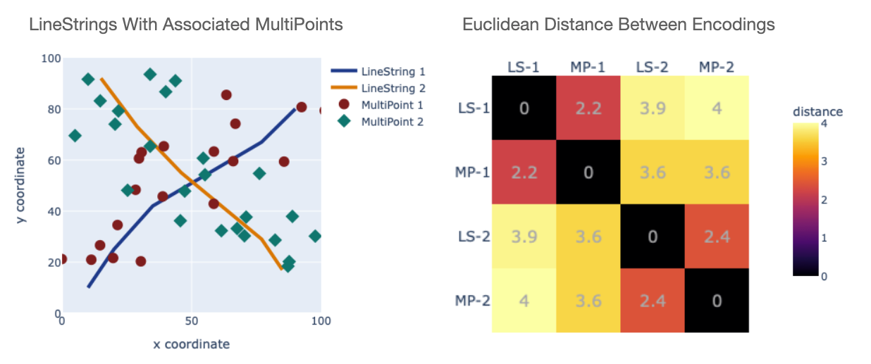
The plot on the right shows the Euclidean distance between the MPP encodings of the four shapes. The distances clearly capture the relationships between the shapes, in that there is a threshold (around 3.0) that would group the pairs that "go together". That is, "LineString 1" lies closer in encoding space to "MultiPoint 1" than to "MultiPoint 2". So using the MPP encoding we can discover spatial similarities and differences among different types of geometries.
Applications of MPP encodings
The concept of positional encodings is widely known in text processing. The idea is that the transformer architecture (Vaswani17) – the backbone of virtually all large-scale AI systems – has the property that its output is "permutation equivariant" with respect to its input. The practical implication is that without augmentation it has trouble deriving meaning from the precise order the input tokens. So transformers typically use positional encodings to capture word order. As was discussed above for the geospatial case, these encodings come from deterministic algorithms rather than being learned. For example the approach in Vaswani17 uses sinusoidal functions of word order, which are then added to the tokenized input to a transformer layer. The alternative approach of "rotary position encoding" applies rotations to encoded tokens based on their order (Su17).
A similar type of augmentation would benefit geospatial applications. For example a problem that has received a lot of attention is "geographical embedding", in which one tries to define embeddings that capture a wide range of information about a location, such as demographics, weather, geophysical attributes, and so on. For example Wozniak21 characterize the properties of H3 cells based on a selection of map objects that they contain. They describe their method as being analogous to a "bag-of-words" model, in which the detailed spatial relationships among selected entities are not specified, beyond the fact that they lie in the same H3 cell. An MPP encoding could serve to augment such approaches in the same way that text positional encodings augment text data in AI models, building in explicit information on how the input objects relate to one another spatially.
Summary and what's next
This has been a quck summary of a positional encoding strategy that offers a lot of potential for GeoAI applications. Multi-Point Proximity can be computed for any type of geometry, and can be built to cover any spatial region. The method takes any collection of shapes and coverts them into conformable representations that can be fed into machine learning models. And we have demonstrated that the encoded values capture important spatial properties of the objects that they encode. So the method has good potential as a Positional Encoding step in an embedding pipeline.
Follow-up posts will go into different aspects of this method's properties and potential uses. Subjects to be covered are:
- Properties of MPP encoding, including continuty and resolution dependence, and how it fits into the general context of Spatial Representation Learning.
- How MPP encodings can be fed into ML and AI models, essentially providing a modality that complements or relplaces raster / image representations.
- Use of sparse vector representations and alternate reference point selections, opening up the possibility of MPP encodings for global-scale applications.
Code and notebooks
A python package named geo-encodings implements MPP encoding, in addition to some other things that I will write about in later posts.

The associated github repo also contains the notebooks that were used to produce the figures above.
Comments and contributions are welcome!
Revision History
- April 6, 2025: Initial release
- April 17, 2025: Added this "revision history" section.
References
"The world's first GIS textbook": Burrough, P. A. Principles of geographical information systems for land resources assessment, Oxford [Oxfordshire] : Clarendon Press ; New York : Oxford University Press, 1986.
Mai22: Gengchen Mai, Krzysztof Janowicz, Yingjie Hu, Song Gao, Bo Yan, Rui Zhu, Ling Cai, and Ni Lao, A review of location encoding for GeoAI: methods and applications, International Journal of Geographical Information Science, Volume 36(4), Jan 2022.
Mai24a: Gengchen Mai, Yiqun Xie, Xiaowei Jia, Ni Lao, Jinmeng Rao, Qing Zhu, Zeping Liu, Yao-Yi Chiang, Junfeng Jiao, Towards the next generation of Geospatial Artificial Intelligence, International Journal of Applied Earth Observation and Geoinformation, Volume 136, 2025, 104368, ISSN 1569-8432.
Mai24b: Gengchen Mai, Xiaobai Yao, Yiqun Xie, Jinmeng Rao, Hao Li, Qing Zhu, Ziyuan Li, and Ni Lao. 2024. SRL: Towards a General-Purpose Framework for Spatial Representation Learning. In Proceedings of the 32nd ACM International Conference on Advances in Geographic Information Systems (SIGSPATIAL '24). Association for Computing Machinery, New York, NY, USA, 465–468.
Su17: Jianlin Su and Yu Lu and Shengfeng Pan and Ahmed Murtadha and Bo Wen and Yunfeng Liu. 2023. RoFormer: Enhanced Transformer with Rotary Position Embedding}, arXiv: https://arxiv.org/abs/2104.09864.
Vaswani17: Ashish Vaswani, Noam Shazeer, Niki Parmar, Jakob Uszkoreit, Llion Jones, Aidan N. Gomez, Łukasz Kaiser, and Illia Polosukhin. 2017. Attention is all you need. In Proceedings of the 31st International Conference on Neural Information Processing Systems (NIPS'17). Curran Associates Inc., Red Hook, NY, USA, 6000–6010.
Wozniak21: Szymon Wozniak and Piotr Szymanski. 2021. hex2vec - Context-aware embedding H3 hexagons with OpenStreetMap tags. GEOAI ’21, November 2–5, 2021, Beijing, China.
Yin19: Yin, Y., et al., 2019. GPS2Vec: Towards generating worldwide GPS embeddings. In: ACM SIGSPATIAL 2019. 416–419.
Comments ()