Masked Geospatial Modeling: Towards Vector-Mode Regional Geospatial Embeddings
Think about what it takes to solve this problem:
Fill in the blank:
I took my ___ for a walk because he was barking so much.
Most people would guess that the missing word is "dog", but how does one infer that? For starters, you need to understand the structure of the laguage, the fact that "he" refers to both the missing word and the thing that was barking. You might infer that the speaker has some control over the thing that was barking, as one typically has over a pet dog. You might also know that dogs usually like walkies, and are keen to vocalize their desires. Put all that together and "dog" seems pretty likely.
In short, you made use of a lot of prior knowledge and understanding. That is why this type of problem is the basis for training many state-of-the-art Artificial Intelligence models. In Masked Language Modeling (MLM), AI models guess the values of missing words in their input. BERT [1] and its many descendants [2, 3, 4, etc.] are probably the most celebrated examples. You take a huge corpus of text, and randomly mask out some of the words. For every masked word, a model computes a probability distribution over all words in the language, indicating how likely each is to be the missing one. The model would yield some probability that the missing word was "dog", but it would also give a probability for "cat", "doorknob", "shoelace", "yellow", and every other word in the language. Although "dog" would probably get the highest score, "dachsund" might also have some non-trivial probability, or "furbaby". By looking at billions of sentences, the model learns to estimate these probabilities well based on the surrounding text.
Of course a model that guesses missing words is only useful for a narrow range of applications. But to do that task well, it has to capture relationships in the structure of the language and the semantic content of the words. One trained, we can discard the model's final procesing layers, leaving us with an internal representation that presumably captures the meaning of input sentences in some abstract way. That representation, or "embedding" for the sentence, can be fed to a wide variety of other tasks, like sentiment analysis, summarization, and question answering.
Word order matters
An essential feature of any text-based AI model is positional encoding. Modern AI models virtually all use the transformer architecture [5], which has the property of being permutation equivariant. That means that if you randomly permute the inputs, you get the same outputs permuted in the same way. To see why this is a problem, consider two sentences.
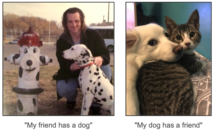
My friend has a dog.
My dog has a friend.
They contain the exact same words, but in a different order, and in language order matters. Shuffling the words around can completely change what we are talking about. Presumably "my friend" and "my dog" are different beings, so the sentences above are not just a re-ordering of the same concepts.
In this case, a transformer would only move the token encodings around, rather than potentially coming up with entirely new encodings and relationships among them. Such a model might have difficulty distinguishing the different shades of meaning in the two sentences.
Positional encodings are the solution. When text is fed to an AI model, the input also includes information that essentially says "this is the first word, this is the second word, ..." and so on. One does not use simple indices (1, 2, 3, ..) but rather other methods that represent order in a way that AI models can exploit easily. [5, 6]
Applying the MLM concept to geospatial data
But this is "Odyssey Geospatial Blog", so this must lead to geospatial analysis somehow.
In an earlier series of posts, I talked about "geometric encoding", which means coming up with ML-compatible representations of geometric shapes so that they can be used as input to Machine Learning (ML) models. A particularly useful method is Multi-Point Proximity (MPP) encoding [7]. The MPP encoding of a geometric object is defined by computing the scaled distance between the object and a set of points within some reference frame. Here is an example.
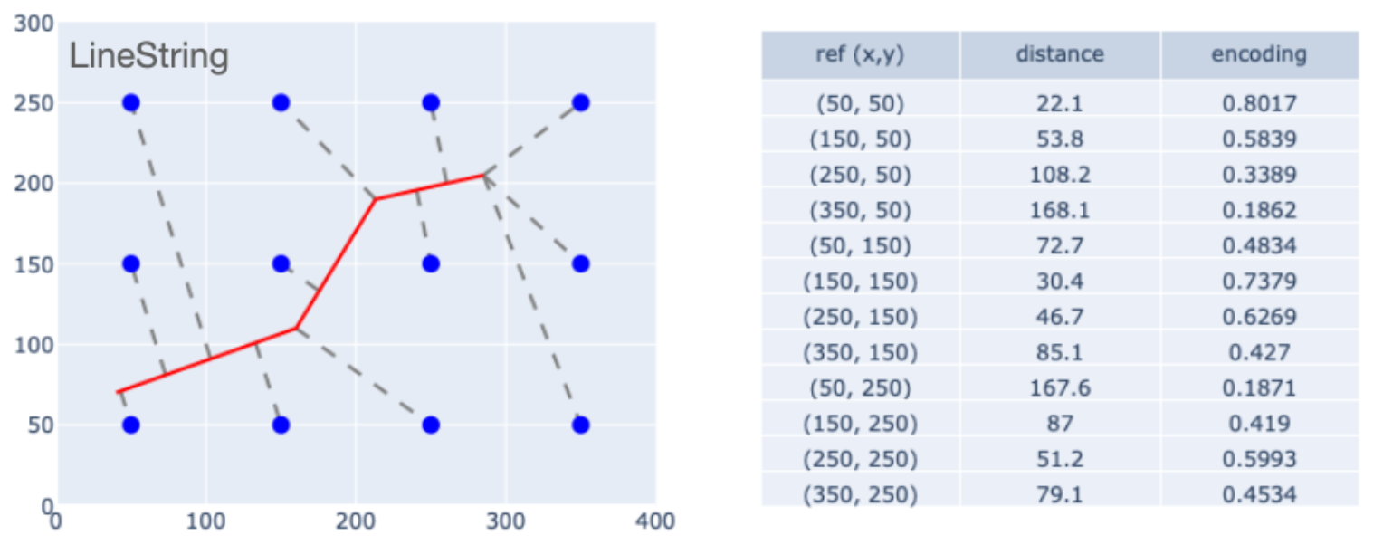
Here we have a LineString object within a $400 \times 300$ reference frame. There are 12 reference points, each of which lies a distance $d_i$ from the line (based on the line's closest point). If we take those distances and scale them as $e_i=\exp -d_i/s$, you get the last column of the table, which is a vector that encodes the shape. ($s$ is a scaling factor.) Although this example shows a LineString, the method applies just as well to Points, Polygons, and multipart geometries. So any shape in the reference frame has its own MPP encoding.
In other posts, I have shown that MPP encodings can capture some essential geometric properties of encoded shapes, can represent pairwise spatial relationships between objects, and can be used to parameterize ML models of geophysical phenomena. In short, MPP encoding is a really useful technique that enables all kinds of geospatial ML / AI applications.
Cutting to the chase, the key point here is that geometric encodings for geospatial problems are analogous to positional encodings for text processing.
Suppose you want to know something about a region, such as its suitability for siting a certain type of business, or whether it would be a nice place to spend an afternoon. You might start by looking at a map and asking questions. Do the local roads make it easy to get to? Are there places to park? Is it near the beach? Will I be able to find coffee shops with good wi-fi?
If you wanted to train a model to characterize neighborhoods, you could make a list of the local geospatial entities, summarize their properties in some ML-compatible form, and train models to distinguish residential neighborhoods, dense urban areas, commercial districts, and so on. Such models exist [8] and have shown some success. But they often don't specify the spatial relationships between entities. In this way they are analogous to "bag-of-words" models used in some older text processing applications, where an article might be described with a histogram of the words that it contains, without accounting for the order in which those words occur.
Just as positional encodings overcome the limitations of the bag-of-words approach (as well as limitations of the transformer architecture), so geometric encodings offer a way around a "bag-of-geospatial-objects" approach.
The analogy extends easily to the concept of Masked Language modeling. A sentence or paragraph is analogous to a geographical region. Words or tokens are analogous to geospatial entities (road segments, buildings, coastlines, etc.) Positional encodings are analogous to geometric encodings. Masked modeling problems have the form:
- Text: Predict the word with this positional encoding given the other words in the sentence.
- Geography: Predict the type of object with this geometric encoding given the other geospatial entities in the region of interest.
This motivates an approach that we might call "Masked Geospatial Modeling" (MGM). A well trained MGM would have internal representations capture the nature and relationships of geospatial entities in a region. And presumably those internal representations could be used for a variety of other tasks.
The following sections describe a study that aims to prove out this concept.
A geospatial dataset for MGM
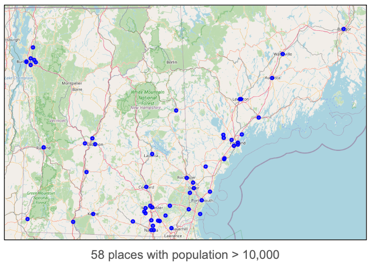
Our MGM will take as input lists of map objects for 1000m $\times$ 1000m "tiles". Ideally dataset would include samples from all over the world, since the structure of objects within a region can vary a lot from place to place. But to keep things manageable for this proof-of-concept study, we will instead sample from a limited geographical region. Map data will come from the northeastern United States, specifically cities and towns with a population of at least 10,000 in the states of Vermont, New Hampshire, and Maine. There are 58 such places.
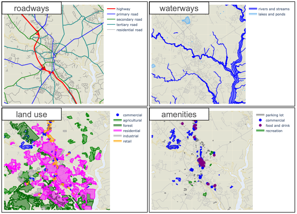
For each such place, I used OpenStreetMap (OSM) to extract geospatial features for a 10 km $\times$ 10 km square. OSM includes a large variety of features, but for this study we will use 22 types falling into into five categories.
- Roadways: highways, primary roads, secondary roads, tertiary roads, residential roads.
- Railways: railroad tracks, rail stops.
- Water: rivers and streams, lakes and ponds.
- Landuse polygons: agricultural, commercial, forest, industrial, recreation, residential, retail, meadow.
- Amenities: parking lots, commercial sites, eating and drinking establishments, recreational sites.
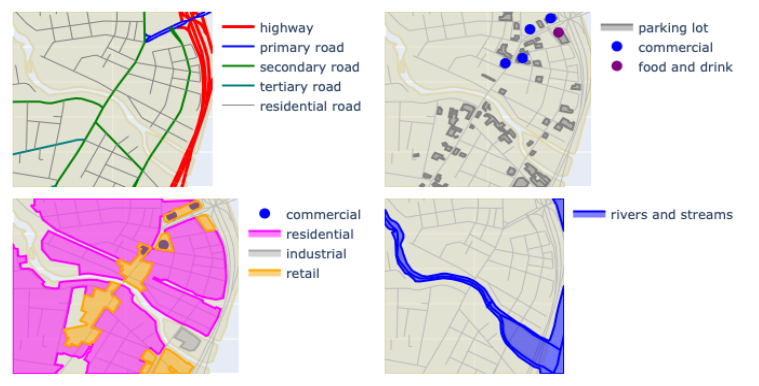
This is what some of these feaures look like for one of the 58 study regions (Dover, New Hampshire).
It's worth noting some complications in OpenStreetMap data. Specifically there is no guarantee for features to be defined consistently from place to place. One city may have a fairly complete delineation of its residentail zones while another has only spotty coverage. Or different contributors may describe similar features using different metadata tags. Such differences are probably minimized by our approach of pulling all data from the same general region, but they still may affect results.
I divided each 10 km $\times$ 10 km area into a set of 1 km $\times$ 1 km tiles. Successive tiles were shifted by 500 meters, so they overlap, which gives us a kind of data augmentation. I took the intersection of all features in the area with each tile, and retained tiles that contained at least 20 features. This yielded a dataset of 19,350 tiles, each containing between 20 and 300 features.
Feature encoding
The data for each tile consist of Point, LineString, Polygon, and MultiPolygon objects, each represented in Well-KnownText (WKT) format. While a dataset with such variable structure is difficult to incorporate into ML / AI models, MPP encodings provide a consitent representation for all features, simplifying their use as model inputs.
For each tile, I defined a set of reference points with a spacing of 50 meters, which gives us 400 reference points per tile. For each geospatial entity, we compute its closest-point distance to each reference point, and apply the negative exponential scaling noted above. That yields a 400-element geometric encoding for each entity in the tile.
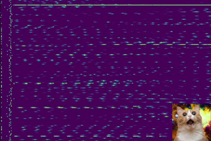
The class label of each entity is encoded as a 22-element one-hot vector correpsonding to the 22 possible types of geospatial entities. The final feature vector of an entity in the dataset is a concatenation of this one-hot vector with its geospatial encoding. For example the tile containing these 208 elements
has an encoding that looks like this.
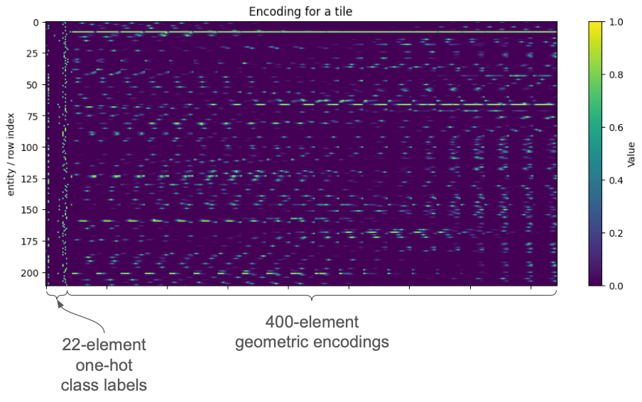
The block on the left consists of the MPP encodings of each entitity. The block on the right consists of the one-hot vectors. So ultimately a tile containing N entities is represented by a N $\times$ 422 matrix.
Building the masked geospatial model
If you are familiar with text-based ML/AI models, then the benefits of this geospatial encoding should be obvious: it is the right format for input to a transformer. Similarly to text processing, each row represents an entity (a word or token for text, a geospatial entity in our case), and the whole matrix represents a unit for the model to consider (a sentence in text, an area of interest here). And as text position encodings indicate how the entities relate to one another, so the geometric encodings represent the spatial properties of the entities being considered.
The 19,350 tiles were divided into training and validation sets. The split was done based on the 58 regions for which we assembled geospatial data. That is, all of the tiles for a region were either assigned to the training set or the validation set. This is a common type of trick in geospatial analysis, since spatial autocorrelation between nearby tiles could otherwise contaminate the purity of the training / validation split. 80 percent of the regions were used for training and 20 percent for testing.
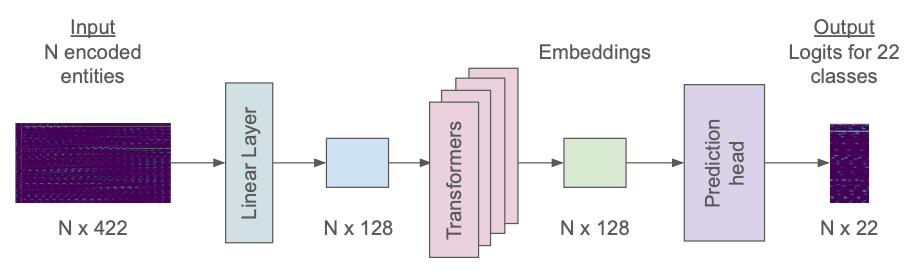
The model uses a basic transformer-based architecture. It consists of an initial linear layer that projects the input 422-dimensional vectors into a space of 128 dimensions. After processing through 4 transformer layers, the resulting embeddings are passed to a classification head yielding logits for the 22 possible classes. These are used to compute cross-entropy loss for optimization.
That is how the model would process a single tile. During training we use batches of 16 tiles, and pad the smaller ones with zeros to match the size of the largest.
Masking is applied during training. When a tile is used in a training batch, we mask a random sample of 15% of the class labels. Masking means replacing the one-hot vector for a sample with a vector consisting of all zeros. We use a technique from most text-based MLMs, and apply the sampling dynamically, so that the set of masked entities varies from epoch to epoch. This better exploits the information in each tile, and makes it very unlikely for the model to over-fit its training data.
Importantly, the masking applies only to the one-hot label for an entity. Its geometric encoding remains unmasked. Essentially we are asking the model, "what do you think the label might be for an object with this geometric encoding?" It is the task of the model to look at the masked encodings, compare them to the encodings of all other entities in the tile, and make its best guess as to what the masked entities are.
The model has about 1.05 million trainable parameters. I trained it via a Google Colab notebook, using one T4 GPU. I trained it for 80 epochs, which took less than one hour.
Performance of the masked geospatial model
To visualize performance, we can compute the average predicted probabilities (the softmax-scaled logits) for each class, grouped by the actual class label, for the masked entities in the validation set.
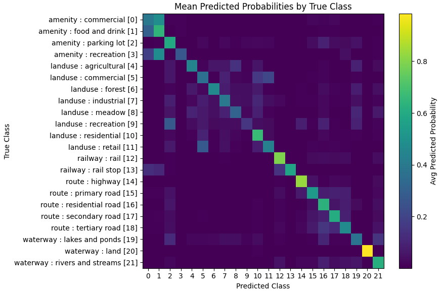
Clearly this is working to some extent. In all cases the true class gets the highest predicted probability. There is some tendency for confusion between "commercial" and "food and drink" establishments. Think of this as the model saying something like "this entity is probably a commercial establishment, but might be a restaurant or bar". That's probably due to the fact that such types of businesses often occur in the same general vicinity. So perhaps a bit of ambiguity in the predictions is warranted.
As a quick ablation study, I trained a version of the model without the transformer layers. Because transformer layers are sensitive to relationships among all entities, they let the model consider the collection of inputs as a whole, capturing their relative placements and spatial relationships. If we delete these layers, we are essentially predicting class probability based the geometric encoding of each entity in isolation. This table gives the overall F1 score, and the top-k accuracies for both models. The top-k accuracy is the fraction of cases for which the true label is among the k with the highest estimated probabilities.
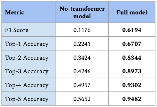
All metrics show that the transformer layers add significant predictive power. This suggests that the model is learning to interpret the geometric encodings and relationships among them, extracting information about the ensemble of entities in an area. That's exactly what we would hope for when trying to compute regional embeddings.
Discussion
The model here is limited in scope. It could be applied to problems involving similar collections of geospatial entities, for areas of a comparable size as the tiles used as training instances. Given the constrained geospatial region from which training samples were drawn, performance would likely decline for other regions of the world, where the typical spatial patterns differ from those of the northeastern United States. There is a long way to go before this could serve as a general "foundation model".
Hovever, our model could not solve the MGM problem without developing an implicit understanding of spatial relationships among objects, as represented by their geometric encodings. That suggests that combining MPP encoding with MGM yields a viable pipeline for developing geospatially aware ML/AI.
But as noted above, solving the MGM problem is mostly a means to an end, that end being creation of embeddings that capture spatial relationships and patterns. In the figure of the model architecture, those embeddings would correspond to the internal representations coming out of the transformer layers. Presumably they capture spatial properties of the input, and could serve as input for downstream tasks other than missing label prediction. Such applications might include site suitability assessments, summary descriptions of neighorhoods, or answering questions about the area.
Readers familiar with text-based foundation models may have noticed an elephant in the room, which complicates the use of these transformer outputs as general-purpose embeddings: our model is permutation-equivariant. If you shuffle the order in which geospatial entities are presented to the model, you get a corresponding shuffling of the results. For the MGM problem this is good: the predictions should not vary just because we re-order the inputs. But this is undesirable when creating general-purpose embeddings, where we want the transformation to be fully permutation-invariant, yielding the exact same result regardless of input ordering.
The inputs to geospatial models like this are essentially set-valued. That is, each input is a mathematical "set" object – a set of encodings for the entities in an area – with no inherent notion of order. While geopatial entities have important relationships to one another, such as proximity, containment, adjacency, and intersection, the order in which they are presented to the model should be irrelevant. This is an important contrast with text-based models, in which the linear ordering of input tokens contains critical information for their interpretation. So this highlights a unique feature of geospatial applications.
While spatial relationships are captured by the MPP encodings, assuring permutation invariance has to be addressed via the structure of the model. Some extremely relevant work has been done on building models (particularly transformers) with set-valued inputs, for which a logical requirement is for the model to be fully permutation-invariant [9]. The most straightforward way to make the output of a transformer permutation invariant is to apply a reduction like the (weighted) sum or mean of the inputs.
The next post in this series will go into a lot more depth on that point, and will develop an extra training step to render MGM embeddings permutation invariant, making them more suitable as inputs for downstream processing.
Thanks for reading!
I hope you have enjoyed this topic. Comments are more than welcome, so feel free to share what you think, whether it's appreciative or critical.
Code
Notebooks for this material can be found here:
AI disclosure
AI tools were prompted for initial drafts of neural network code for masked geospatial modeling, and assisted generating the maps above. All text was produced by the author.
References
[1] Devlin, J., Chang, M.-W., Lee, K., & Toutanova, K. (2019). BERT: Pre-training of Deep Bidirectional Transformers for Language Understanding. In Proceedings of the 2019 Conference of the North American Chapter of the Association for Computational Linguistics: Human Language Technologies (pp. 4171–4186). https://arxiv.org/abs/1810.04805
[2] Sanh, V., Debut, L., Chaumond, J., & Wolf, T. (2019). DistilBERT, a distilled version of BERT: smaller, faster, cheaper and lighter. arXiv preprint arXiv:1910.01108. https://arxiv.org/abs/1910.01108
[3] Beltagy, I., Lo, K., & Cohan, A. (2019). SciBERT: A Pretrained Language Model for Scientific Text. In Proceedings of the 2019 Conference on Empirical Methods in Natural Language Processing (EMNLP) (pp. 3615–3620). https://arxiv.org/abs/1903.10676
[4] Lee, J., Yoon, W., Kim, S., Kim, D., Kim, S., So, C. H., & Kang, J. (2020). BioBERT: A pre-trained biomedical language representation model for biomedical text mining. Bioinformatics, 36(4), 1234–1240. https://doi.org/10.1093/bioinformatics/btz682
[5] Ashish Vaswani, Noam Shazeer, Niki Parmar, Jakob Uszkoreit, Llion Jones and Aidan N. Gomez, Lukasz Kaiser and Illia Polosukhin (2023). Attention is all you need. https://arxiv.org/abs/1706.03762
[6] Jianlin Su, Yu Lu, Shengfeng Pan, Ahmed Murtadha, Bo Wen and Yunfeng Liu (2023). RoFormer: Enhanced Transformer with Rotary Position Embedding. https://arxiv.org/abs/2104.09864
[7] John Collins (2025). Multi-Point Proximity Encoding For Vector-Mode Geospatial Machine Learning. https://arxiv.org/abs/2506.05016.
[8] Szymon Woźniak and Piotr Szymański (2021). hex2vec: Context-Aware Embedding H3 Hexagons with OpenStreetMap Tags. In Proceedings of the 4th ACM SIGSPATIAL International Workshop on AI for Geographic Knowledge Discovery (SIGSPATIAL ’21). https://arxiv.org/abs/2111.00970
[9] Juho Lee, Yoonho Lee, Jungtaek Kim, Adam R. Kosiorek, Seungjin Choi and Yee Whye Teh (2019). Set Transformer: A Framework for Attention-based Permutation-Invariant Neural Networks. https://arxiv.org/abs/1810.00825
Comments ()