Predicting Rates Of Rare Events

A few months ago I was working in my home office when the house started to shake. At first I thought maybe a big tree fell somewhere nearby – it happens sometimes in the forested area where I live. But the rumbling went on for about 10 seconds, too long to be a falling tree. After walking around the house to see if anything was damaged, a thought occurred to me. So I went back inside and dialed up a USGS web site, and – yep – we had just had an earthquake.

I live in New Hampshire. New Hampshire doesn't get earthquakes, or so I thought. They happen in places like California or Chile or Japan, not along the quiet, tectonically stable east coast of the US. But in fact earthquakes do happen in a lot of places where you wouldn't expect, wherever some pressure builds up in the earth's crust, causing some old fault line to shift a bit.

Suppose that somebody was interested in exactly how often earthquakes occur in a given area. And to collect data, that researcher picked a few locations – say geohash boxes or H3 grid cells of a certain size – and counted the number of times each contained an earthquake epicenter over the course of a year. Those counts could serve as "truth" for modeling earthquake rates as a function of, say, local geological properties, proximity to fault lines, and so on.

[If this sounds familiar, then maybe you read my recent story on Medium. I'll add the same disclaimer here as I did there: I'm not a geologist, and there are well established ways to estimate earthquake rates. In fact the scenario is a bit contrived: there already exist systems that reliably locate earthquake epicenters globally. But I'm going somewhere with this.]

The key question is: what would you want the model to predict as an earthquake rate for where I live? The data say that we got one earthquake this year, so a naïve calcualtion of the local rate is 1 / year. But the actual rate is a lot lower, like one every 100 years or more. And how about the next county over? They got none this year, so is their true rate zero? Probably not – they might have some old fault line that could become active at some time.

The problem is that we are trying to predict the rate of rare events. For any area for which we are keeping count, the most likely number of observations is zero. A small fraction will have a value of 1, and an even smaller fraction will have values of 2 or more The sparsity of the phenomenon means that whatever number we observe will not be a very good estimate of the true rate. Getting a precise estimate would require observations over an impractically long time period, like a thousand years.

Building a model to predict the rate of rare events

This is a regression problem. Since rates represents expected long-term averages, they need not be integers. For example a rate could be 0.01 events per year, if the long-term expectation is one event every century.

The theoretical foundations of some regression models demand that measurement errors have certain properties, such as having zero mean, being normally distributed, or having the same variance across the dataset. None of those are likely to be true in our case. Suppose we are trying to estimate a set of rates whose true values are on the order of 0.1 events per year. The observed counts would be zero in most cases – almost always less than the true value. So there would be a bias in the measurement error.

We can still build a solid theoretical foundation for our model by framing the problem a bit differently. Consider a set of $N$ areas $\{i \in 1..N\}$ for some period of time (say a year), and count the number of times the event of interest (an earthquake) occurs. Call the counts $C = \{c_i\}$. Instead of thinking of these counts as yielding reliable rate estimates, assume that there are underlying rates $R = \{r_i\}$ that determine the count $c_i$ for each location $i$. Or in other words, $c_i$ is a realization of a random varable that has $r_i$ as a parameter.

The most common choice for a probabilistic model in cases like this is the Poisson distribution, which gives the probability of observing some count given the underlying rate at which it occurs. \[P(c; r) = \frac{e^{-r}r^c}{c!}\] That gives us a workable relationship between what we observed and what we want to estimate.

To estimate the underlying rates $r_i$ we can use a set of features $F = \{f_i\}$, which might be things like the dominant type of bedrock at locaiton $i$, its proximity to fault lines, and so on. That is, our model looks like \[\hat{r_i} = M(f_i; \theta)\] The model has some parameters $\theta$; if the model is a neural network then $\theta$ are the weights to be learned via gradient descent.

To optimize the model, we can use the principle of maximum liklelihood, and pick the set of parameters such that the the rate predictions $\hat{r_i}$ yield the largest possible joint probability of observing the set of counts from our observations. \[\max_\theta \prod_i P(c_i; \hat{r_i}).\] Or in other words, \[\max_\theta \prod_i \frac{e^{-\hat{r}}\hat{r}^c}{c!} \] where I have dropped the subscripts for clarity.

Suppose we are building a big model, estimating rate parameters for a million different locations. In that case, the product in that last equation can not be calculated reliably by a computer. If every rate parameter had a value on the order of 0.1, then the total value of the product would be somewhere around $1 * 10^{-1,000,000}$. Using a common trick, instead of trying to maximize a product, we instead try to minimize the negative of its logarithm. Since the logarithm is a monotonic function, we get the same answer either way. So the product becomes a sum, and the new problem is \[\min_\theta\sum-\log\frac{e^{-\hat{r}}\hat{r}^c}{c!}.\] After some algebra, that becomes \[\min_\theta\sum_i\hat{r_i} - c_i \log(\hat{r_i})+\log(c_i!).\] That last equation is called the Poisson loss function or the Poisson negative log likelihood. It is recognizable as a loss function because its inputs are a set of predictions $\hat{r_i}$ and a set of true values $c_i$, and it gets smaller as the model gets better. Since the last term $\log(c!)$ is not a function of the model's parameters, it doesn't influence gradient descent and is sometimes omitted. There are implementations of this function in all popular neural network frameworks, like keras and pytorch.

In summary, we now have a solid theoretical foundation for building a model to predict rates of rare events, in which our observations do not directly yield good estimates of the true parameters we are going after.

For example

Here is a simple example to illustrate how this works in practice, using a synthetic dataset. All of this uses python and pytorch.

To start, we generate a set of random-valued features. These will be the predictors in our model.

import torch

# Use this many randomly-generate features.
n_features = 5

# Make this many training + validation cases.
n_cases = 10000 

# Create some random-valued features.
features = torch.rand((n_cases, n_features))

That gives us features for 10,000 cases, each of which is a 5-element vector. From here we can define rate parameters as a function of the feature values. This is one of many ways we could do it.

# Define a set of rate parameters as a 
# function of the feature values.
rates = torch.ones(n_cases)
for i in range(n_features):
    random_factor = np.random.random() + 1.5
    random_exponent = 0.5 + np.random.random() * 1.5
    rates = rates * torch.pow(features[:,i], random_exponent) * random_factor

The rates are the parameters that we hope to estimate. In a real-world situation, we would never know their true values, but instead would observe event counts goverened by them. We can generate such synthetic counts like so.

counts = torch.poisson(rates)

Now we have a set of synthetic feature values (features) and a set of synthetic observations (counts), that we can use to estimate rate parameters (rates) which would be unknown in practice, but which we know here because we generated the data.

This is what the synthetic rates and counts look like.

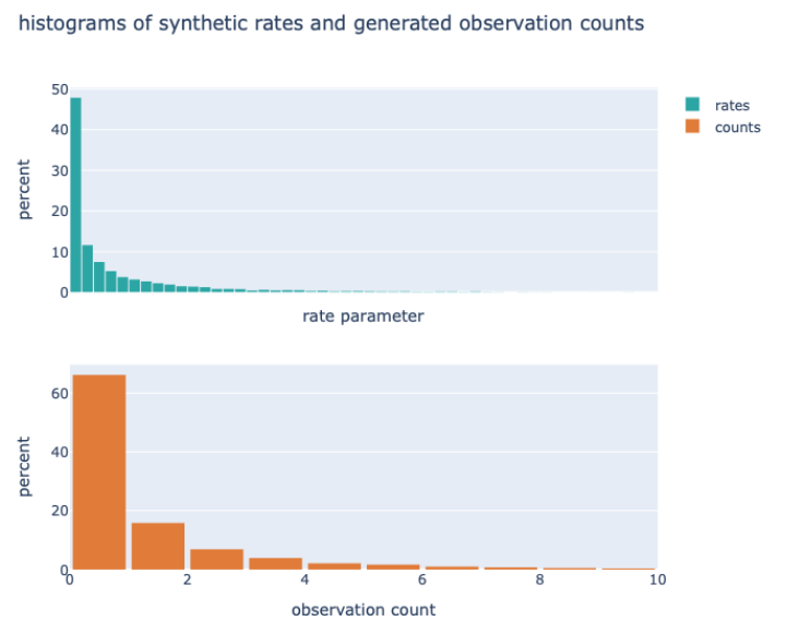
The rate parameters are relatively small, with about 48% being less than 0.2 (think of the units as events per year). As a result, about 68% of all counts are zero.

We can split up the synthetic data into training and validation subsets like so.

# Train / Validation split
dataset = TensorDataset(features, counts)
train_size = int(0.8 * len(dataset))
val_size = len(dataset) - train_size
train_ds, val_ds = random_split(dataset, [train_size, val_size])
train_loader = DataLoader(train_ds, batch_size=1000, shuffle=True)
val_loader = DataLoader(val_ds, batch_size=1000)

Then we can build a simple pytorch model to predict a single value (the rate parameter) given the input features.

# Define the model.
class PoissonRatePredictor(nn.Module):
    def __init__(self, hidden_size):
        super(PoissonRatePredictor, self).__init__()
        self.fc1 = nn.Linear(n_features, hidden_size)
        self.fc2 = nn.Linear(hidden_size, hidden_size)
        self.out = nn.Linear(hidden_size, 10)
        
    def forward(self, x):
        x = F.relu(self.fc1(x))
        x = F.relu(self.fc2(x))
        x = self.out(x)
        rate = torch.exp(torch.sum(x, dim=1)) 
        return rate

model = PoissonRatePredictor(hidden_size=32)

This is mostly a simple 2-layer fully connected model, except for one small flourish: the final layer predicts 10 values, which are then summed and passed through a torch.exp function to yield a single rate estimate. This assures that all predictions from the model are positive. That not only makes logical sense since we are predicting rates (which can't be negative), but is also necessary in our scenario because the Poisson loss function is only defined for positive inputs.

Speaking of the Poisson loss function, pytorch makes it really simple to use for model training.

loss_fn = nn.PoissonNLLLoss(log_input=False, full=False) 
optimizer = torch.optim.Adam(model.parameters(), lr=0.001)

for epoch in range(100):
    model.train()
    total_train_loss = 0
    for xb, yb in train_loader:
        pred = model(xb)
        loss = loss_fn(pred, yb)
        optimizer.zero_grad()
        loss.backward()
        optimizer.step()

And that does it. We get a trained model that predicts rates given features and counts. Let's take a look at how it performs on the validation dataset.

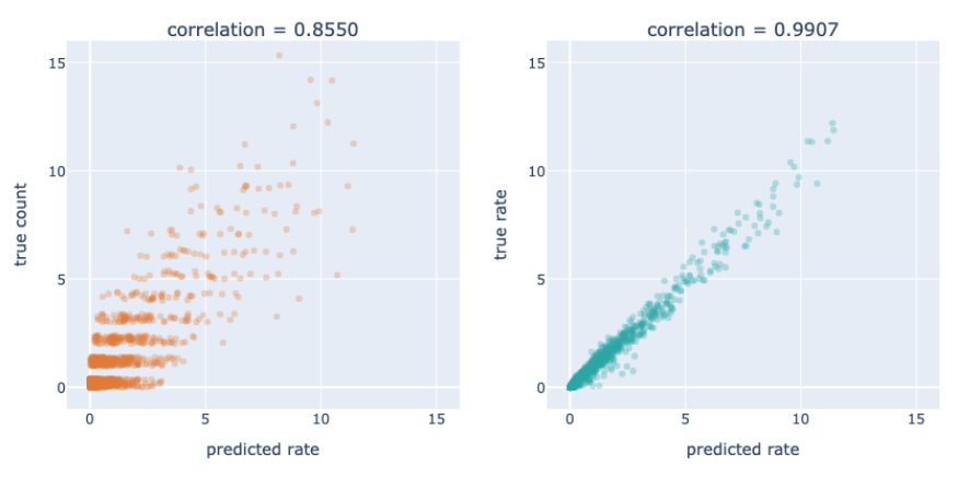
In a real-life situation, we would know the observed counts and the predictions, so the best performance plot that we could produce would be the one on the left. Since counts are integers, I have added a bit of randomness to the values to give a better sense of their distribution. There is a good positive correlation, but also a good amount of scatter. That can be attributed to the nature of the data and the framing of the problem. Even if the model were perfect, we would not expect a perfect relationship between these variables because the observed counts only have an indirect relationship to the true rates. But since we are using synthetic data, we do know the "unseen" values of the rate parameters. The plot on the right shows that this model is doing phenomenally well estimating those rates, even if the plot on the left does not fully capture it.

Summary

This post talked about some theoretical issues that come up when trying to predct rates from sparse observations. By framing the problem as maximum likelihood estimation of rate parameters from Poisson-distributed counts, we derived the Poisson loss function, and provided code implementing the idea for training a neural network using synthetic data.

I hope you enjoyed the post. Please feel free to leave comments below – they are always appreciated, no matter how brief or critical. And consider subscribing to this blog for updates on new posts. Thank you for reading!

AI disclosure

I think it would be great to normalize disclosures like this, so here you go:

The use of AI technology in this post was limited to generation of a first draft of pytorch model code, and to choice of color schemes for plotting. All writing was produced by the author using his own brain.

Code

Source code for the analysis above can be found on github.