Properties Of Multi-Point Proximity Encodings
My previous post talked about Multi-Point Proximity (MPP) encoding: the idea that any Point, LineString, or Polygon can be approximately encoded based on its distance to a set of reference points. The post demonstrated that the method captures some key properties of the encoded shapes, and allows them them to be used as input to Machine Learning (ML) and Artificial Intelligence (AI) models.
As a quick recap, say we have a geometry $\mathbf{g}$ (a Point, LineString, etc.) for which we want an encoding. We can lay out a grid of reference points over the region that contains $\mathbf{g}$, and compute a kernel function of the distance between each reference point and the closest point on or in $\mathbf{g}$. Or in math:
\[\mathbf{e} = \mathbf{MPP}(\mathbf{g}) = \Big[ \exp\Big( \frac{-\mathrm{d}(\mathbf{g}, r)}{s} \Big), r \in \mathbf{r} \Big] \]
where $\mathbf{r}$ represents the ordered set of reference points, and $s$ is a tunable scaling factor. $\mathrm{d}(\mathbf{g}, r)$ represents the closest-point distance between a point $r$ and the geometry $\mathbf{g}$. Here is an example for a polygon with a hole.
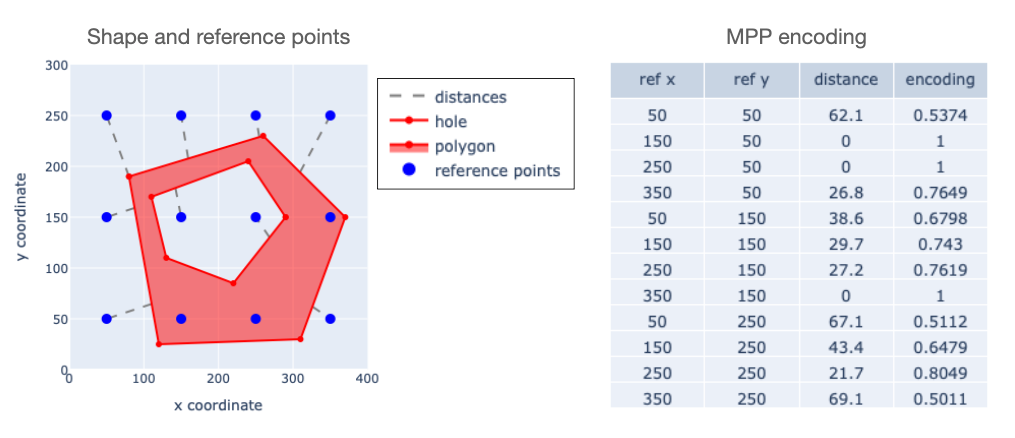
We have laid out 12 reference points witin a $400 \times 300$ region (units are arbitrary, but think of them as meters if it helps), computed their distance to the shape, and scaled the distances according to the equation above. This gives us a 12-element vector that encodes the shape – the last column on the right.
This post will go into more detail about some properties of MPP encodings. I will talk about how the approach fits with the emerging field of Spatial Representation Learning (SRL) discussed in Mai24b. I'll check how MPP encoding performs relative to desired properties for SRL, and will show that it compares favorably against an alternate approach.
Spatial Representation Learning
The goal of SRL is to represent geometric shapes – Points LineStrings and Polygons – in a way suited for use with ML/AI models. That means taking a geometry in some format like Well-Known Text (WKT) or the equivalent, and converting it into a vector that represents its essential properties. The result is an embedding for a shape, which can be seen as the geometric equivalent of embeddings used for text and image processing. Furthermore, the comparison between image embeddings and geometric/spatial embeddings mirrors the dichotomy between raster-based and vector-based approaches to spatial analysis, which has existed since the dawn of GIS.
A framework proposed in Mai22 distinguishes between embedding and encoding. Specifically encoding is the use of a well defined algorithmic approach for picking a number or vector to represent something that is not naturally a numerical entity. In text processing this corresponds to tokenization, where one assigns integer identifiers to words or parts of words making up a vocabulary.
In contrast, embedding is the process of learning a meaningful vector representation for the encoded entity, typically via some self-supervised process. SRL is concerned with the composition of encoding and embedding:
\[\mathbf{e} = \mathrm{PE}(\mathbf{g}) \]
\[\mathbf{m} = \mathrm{NN}(\mathbf{e}) \]
Here $\mathbf{g}$ represents a geometry – a Point, LineString, Polygon, or "Multipart" extension thereof, $\mathbf{e}$ represents the result of Positional Encoding (PE) applied to the geometry, and $\mathbf{m}$ represents the final embedding produced by a trained Neural Network (NN).
In this taxonomy, MPP is a method for encoding, not for embedding.
For an encoding to be a viable option for SRL, it must capture the relevant properties of the shapes that it encodes. Then presumably one can trust later NN learning to preserve and enhance that information for adaptation to ML/AI models. In this post I will focus on the former – the preservation of essential geometric / spatial information in the MPP encoding process, and how it compares to a specific alternative. The specific alternative is...
Discrete Indicator Vector encoding
Both above and in the previous blog post, the reference points used in MPP encoding have been laid out on a regular grid. One could think of these reference points instead as the centroids of a set of non-overlapping rectangular tiles $\mathbf{t}$. Then for encoding a shape, instead of finding the minimum distance from the shape to each $r \in \mathbf{r}$ and applying a kernel funciton, one could assign a value of 1 if the shape intersects each tile $t \in \mathbf{t}$. The encoding is then a vector indicating which of the ordered set of tiles overlap the shape. Call this Discrete Indicator Vector (DIV) encoding.
\[\mathbf{e}=\mathrm{DIV}(\mathbf{g})=\big[1 \enspace\mathrm{if}\enspace \mathbf{g}\cap t \neq\emptyset\enspace\mathrm{else }\enspace 0: t \in \mathbf{t} \big] \]
This really isn't a very novel idea: it's just a simple form of "rasterization", which is a familiar way of using shape data in a raster processing system. But here the focus is a bit different, in that we seek a relatively low-resolution encoding for the purpose of feeding shapes to embedding models or other ML/AI processing. The original paper describing the MPP approach (Yin19) mentions such discrete encoding in passing, as an inferior alternative to the use of a distance-based kernel function, because it would require a very fine grid (and consequently a very large vector) to encode point locations with high fidelity. But here we will use the idea as a baseline for comparison.
Here is an example of how MPP and DIV encoders would handle a given LineString.
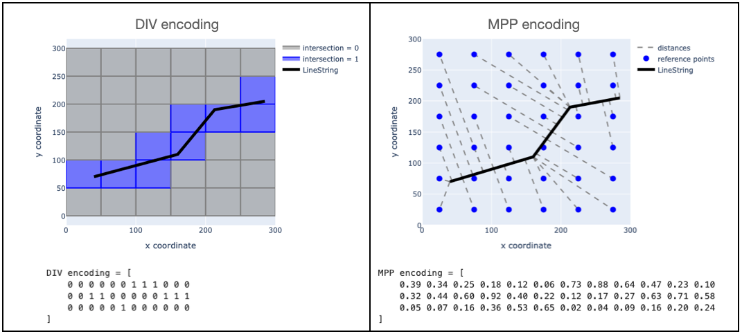
We're using a $6 \times 6$ grid of either tiles or reference points, so each method produces a 36-element vector that tries to capture the relevant properties of the shape. So arguably these two cases have the same "resolution".
The DIV approach gives us a vectors of 1's and 0's indicating which cells the line touches. It's easy to see that any line that passes through the same set of cells would have the exact same encoding. In contrast the MPP result yields a vector whose elements vary continuously. This is actually a very useful property for an encoding to have, as described next.
Continuity of encodings
To demonstrate strength of an encoding method, one could do a couple of different things.
- Apply the encoding method in the context of some larger learning or analysis task, and demonstrate that the results are good, or
- Decide a priori some properties an encoding should have, and check whether they hold for a given method.
I'll get to (1) in later posts, but here I will focus on checking the degree to which MPP and DIV strategies exhibit desirable properties.
One such property is continuity. Informally, one would hope that a slight change to a geometry – a small shift of one of its coordinates or some very small rotation of the shape – would show up as a similarly small change in the encoding. It would not be good for the encoding to show sudden discontinuous jumps in its elements due to slight changes.
As a spoiler, MPP encodings have this property; DIV encodings do not, which shouldn't be much of a surprise as the D in DIV stands for Discrete. While I'll leave it to an expert in computational geometry to prove that definitively, it can be demonstrated in a number of ways. Consider a single Point located somewhere in a $100 \times 100$ region. If we use a tile size / reference point spacing of 25, we get a $4 \times 4 = 16$ element vector from either DIV or MPP. Now suppose that the Point moves along the trajectory shown on the left below. The middle and right plots show the 16 elements of the DIV and MPP encodings respectively, for each point along that trajectory.
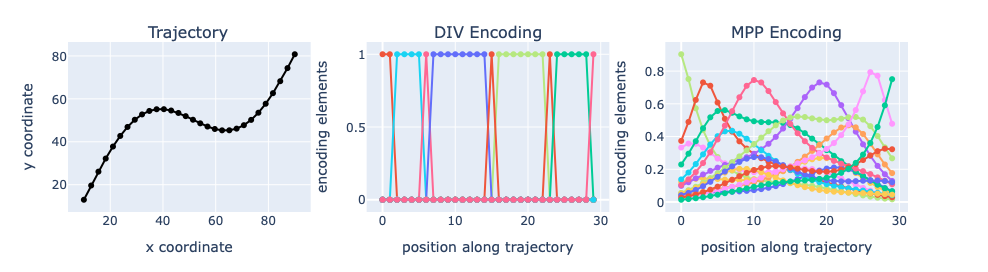
For the DIV encoding, only one element has a value of zero at any time. When the Point crosses into a new tile, there are discrete jumps in the elements for the tile that it leaves and the tile that it enters. In contrast for MPP encoding, each movement along the trajectory is associated with a small change in the value of all elements. This is the "continuity" property that we were hoping for.
There is a situation worth explaining, related to the fact that MPP uses nearest-point distances. If there is a slight shift to the shape or one of its coordinates, the nearest point might jump to a different part of the geometry. The figure below illustrates this for a case with 4 reference points and a LineString object.
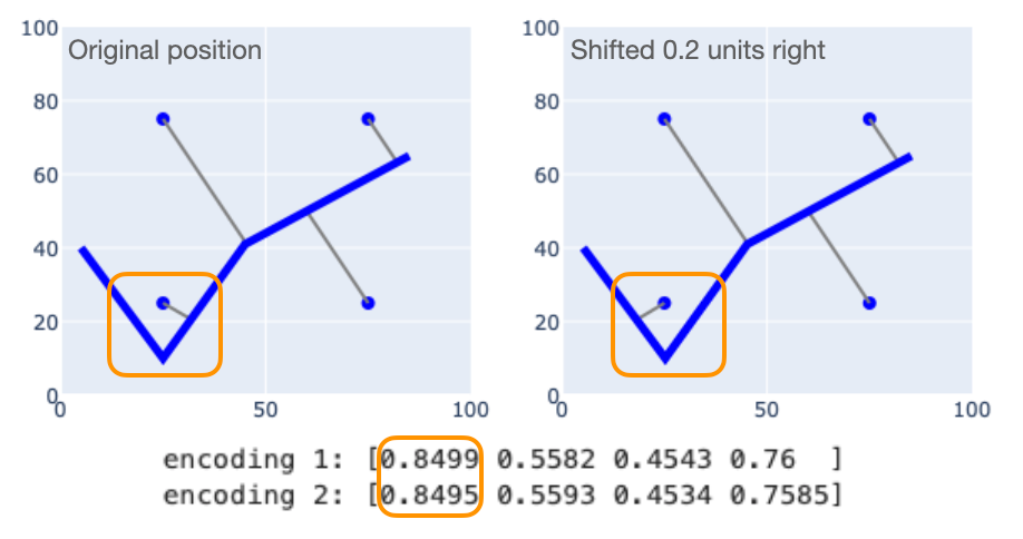
The LineString on the right is a slightly shifted copy of the LineString on the left. Note the reference point at $(25, 25)$: even though the shapes are similar, its closest point jumps from one part of the shape to another. But there is no correspondingly large jump in the associated encoding (the first element). That's because the "jump" happens at the point where the distances to the two different line segments are equal. So while the closest point is different, the distance to that point is about the same. Since only the distance is used in the encoding, the shift does not significantly change its value. So this phenomenon does not invalidate the continutity of the encoding.
Shape-centric representations
A goal stated in Mai24b is for "shape-centric" representations. This refers to the fact that some LineString and Polygon encoding approaches proposed in the literature actually process the list of coordinate pairs that define a geometry. This leads to a couple of possible issues.
- They can be sensitive to the order in which the vertices are specified. For example if one defines the same polygon twice by starting at two different vertices and proceeding clockwise around the border, some encoding methods can yield different results. Instead a desired property is vertex loop transformation invariance, in which changing the starting vertex has no impact.
- They can be sensitive to addition of new vertices that do not actually change the shape. Such an operation can occur frequently in practice: for example if one digitizes a newly constructed road segment that connectds to an existing road segment, one adds a new vertex that does not change its shape. Encoders that process coordinate lists could yield different results in such a case. Here the desired property is trivial vertex invariance, in which such an addition has no effect on the encoding of the original shape.
Since MPP encoding is defined only relative to the shape itself and not to its specific list of vertices, it has both of these properties. So does DIV encoding, for that matter.
Decoding
The framework for Spatial Representation Learning proposed in Mai24b emphasizes the importance of decoding – going from an encoded representation to a geometry in some standard format like WKT. Such an operation would "complete the loop" of GeoAI, letting us take geometries, encode them for AI/ML processing, get results, and convert them back to an explicit geometric representation. Going into the details of how that might be done is a bit out-of-scope for this blog post, but we can demonstrate that MPP encodings preserve information that supports decoding.
The key point is that the elements of an MPP encoding are a monotonic function of distance. So implicitly they encode that distance, in that it's easy to compute it given the encoding: the relationship between distance $d$ and element $e$ is $e = \exp (-d/s)$, so $d = -s \ln e$. What that means is: one can infer the nearest-point distance between any reference point $r$ and the geometry $\mathbf{g}$ that it encodes. And that tells us a couple of things about $\mathbf{g}$:
- Some point on the boundary of $\mathbf{g}$ lies distance $d$ from $r$, and
- No part of $\mathbf{g}$ lies any closer to $r$.
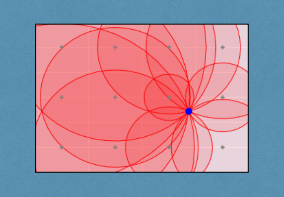
Now suppose we have an encoding for a Point. Look what happens when we plot a circle of radius $d_i$ around each reference point $r_i$.
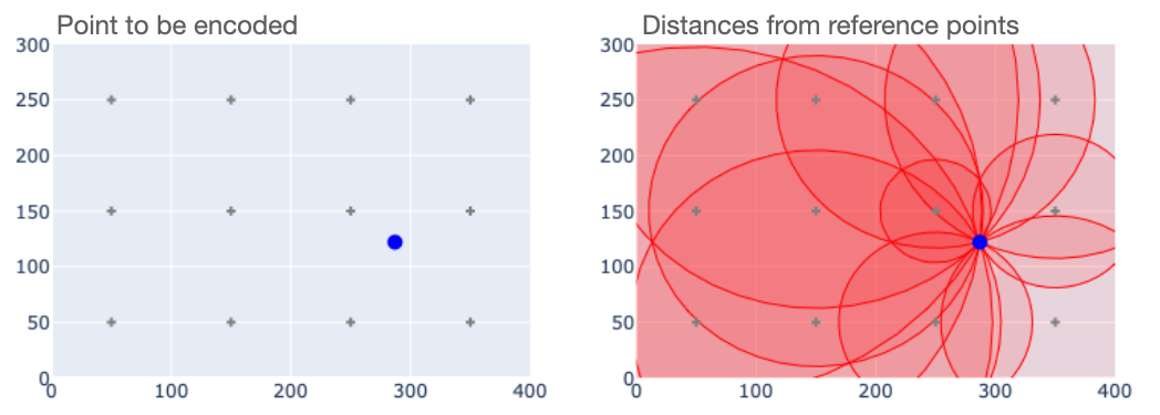
The encoding makes it quite obvious where the encoded Point lies. In fact for Point geometries decoding the location is a simple matter of triangulation, and could in fact be solved in a closed form.
Something similar happens with LineString and Polygon objects.
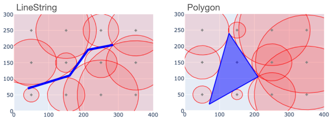
In both cases, the circles around the reference points define a kind of exclusion zone that the decoded geometries have to lie outside of. There is still some ambiguity, in that the exclusion zone does not precisely determine the LineString or Polygon shapes. But if we lay out a denser grid of sample points, things look a bit better. Here is what it looks like if we double the resolution relative to the last figure.
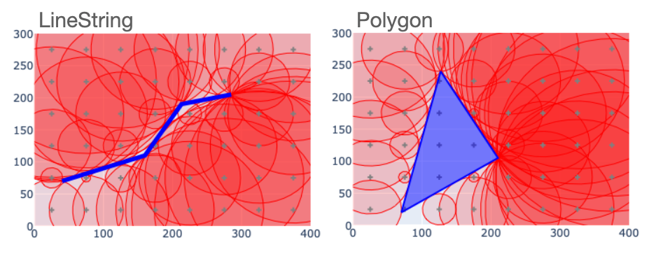
Now the encodings give us a much better idea about where the shapes lie. This tells us that MPP encodings contain information that can be used for decoding, and that the precision of the decoded representation depends on the resolution of the encoding.
This makes it easy to see one of the strengths of MPP over DIV. In MPP, every element of the encoding contains information about the location of the object that it encodes. Even reference points that lie far from the shape tell us something aboout where the shape's boundary lies. And each may exclude a large portion of the region from consideration during decoding.
Summary
This post has looked into some of the features of Multi-Point Proximity encodings, and has shown that they posess some good properties for use in Spatial Representation Learning. In particular MPP encodings are continuous, exhibit desired types of invariance, and encode information that could be used for decoding. While the fideility of the decoding is not perfect, it can be controlled by choosing an appropriate resolution.
In the next post of this series, I'll begin using MPP encodings as inputs to neural network models, and in so doing will illustrate that the encodings capture pairwise geometric relationships among spatial objects. Hope to see you there!
Code
Check out the geo-encodings github repo for an implementation of MPP and DIV encoding. The repo also contains the notebooks used to make the plots above.

And you can always just pip install geo-encodings to start working with them in your python code. I would love to hear about general feedback, proposals for code contributions, and descriptions of any applications that you might think up.
Revision history
- April 6, 2025: Initial release
- April 17, 2025: Fixed some typographical errors.
References
Mai22: Gengchen Mai, Krzysztof Janowicz, Yingjie Hu, Song Gao, Bo Yan, Rui Zhu, Ling Cai, and Ni Lao, A review of location encoding for GeoAI: methods and applications, International Journal of Geographical Information Science, Volume 36(4), Jan 2022.
Mai24a: Gengchen Mai, Yiqun Xie, Xiaowei Jia, Ni Lao, Jinmeng Rao, Qing Zhu, Zeping Liu, Yao-Yi Chiang, Junfeng Jiao, Towards the next generation of Geospatial Artificial Intelligence, International Journal of Applied Earth Observation and Geoinformation, Volume 136, 2025, 104368, ISSN 1569-8432.
Mai24b: Gengchen Mai, Xiaobai Yao, Yiqun Xie, Jinmeng Rao, Hao Li, Qing Zhu, Ziyuan Li, and Ni Lao. 2024. SRL: Towards a General-Purpose Framework for Spatial Representation Learning. In Proceedings of the 32nd ACM International Conference on Advances in Geographic Information Systems (SIGSPATIAL '24). Association for Computing Machinery, New York, NY, USA, 465–468.
Yin19: Yin, Y., et al., 2019. GPS2Vec: Towards generating worldwide GPS embeddings. In: ACM SIGSPATIAL 2019. 416–419.
Comments ()