Recovering Pairwise Spatial Relationships From Geometric Encodings
"A point is that which has no part."
So begins Euclid's Elements, a systematic exposition of the principles of geometry, starting from the most basic definitons, proceeding by logical inference to virtually all that was known about the discipline at the time. It would be hard to find another work that remains a solid foundation of an entire branch of knowledge some 2,300 years after it was written.
Euclid knew that you have to start a discussion by being clear what you are talking about. And even though the notion of a "point" seems intuitive to most people, it truly is a theoretical concept. You can't show somebody a "point" in the real world, because you are invariably showing them something that has at best some small extent. And if it has an extent, then you could in theory divide it in half. So it would have "parts", and theoretical discussions about "points" would not strictly apply to it. But Elements has such enduring importance because it embodies the idea that there are theoretical constructs – things just outside the world of what we can see and touch – which we can understand and reason about, and that serve as models leading to deeper understanding of the real world.
I found myself thinking about Euclid's opening recently, when the question "what exactly is a Point?" came up in a practical situation. I was trying to demonstrate ideas in Spatial Representation Learning, which tries to bring geometric objects into better alignment with Machine Learning and Artificial Intelligence models. Which shows that these kinds of theoretical details about the very foundations of geometry remain relevant in the era of Geospatial AI.
Positional encodings for geometric objects
My last two blog posts talked about an approach to creating positional encodings for arbitrary geometries – ways to represent shapes as vectors of numbers that can be fed to ML and AI models. The idea is that an encoding for a geometry can be defined by applying a kernel function to its distance from a set of reference points [6]. There is a brief recap of the concept in my last post, and a slightly longer discussion in the one before that. The method is called Multi-Point Proximity (MPP) encoding.
The previous posts attempted to show that the approach was a viable candidate for use in SRL, and that the resulting encodings posess at least a few desirable properties.
Once we have a way to represent shapes, we have to be able to do something with them. Perhaps the most basic expression of "do something" is describing relationships between pairs of objects. Such relationships are the fundamental building blocks of spatial analysis. Does this line include this point? Do these two lines cross? Is this polygon adjacent to that one?
This post checks whether such pairwise relationships can be recovered from MPP encodings. That is, we want to be able to say things like "if you start with MPP encodings for two LineStrings, you can say whether they overlap with $x$ precent accuracy". If $x$ is large enough, that strengthens the recommendation for using the method to represent shapes in AI/ML contexts.
Pairwise relationships between shapes
Suppose we have a pair of 2-dimensional geometries. They might be of any type – Points, LineStrings, Polygons, or multipart collections thereof. In how many different ways might those two geometries relate to one another?
262,144 of course.
At least that's the number according to a particular theoretical model used in point-set topology. I'm talking about the "dimensionally extended 9-intersection model", known as DE-9IM for short. The idea is that any geometry has up to three relevant characteristics: an interior $I$, a boundary $B$, and an exterior $E$. If we take a pair of geometries $a$ and $b$, these respective things may or may not intersect with one another. If they do intersect, then:
- If the intersection is a Point, it has dimension 0,
- If the intersection forms a LineString, it has dimension 1,
- Otherwise it has dimension 2.
As for the interior, boundary, and exterior, they are defined by convention for different geometry types.
- Points are defined as having an interior but no boundary. [If we defined a Point as having both a boundary and an interior, it would have separate "parts". Euclid would not be pleased.] The rest of the 2-dimensional universe is the exterior.
- For LineStrings, the boundary consists of the two endpoints, and the interior is the set of all points along the line.
- For a Polygon the boundary is the edge, and the interior and exterior are defined by what the edge encloses.
The relationship between $a$ and $b$ can be described by a $3\times3$ matrix. Each element of the matrix is the dimensionality of the intersection between parts of the two geometries.
\[\mathrm{DE9IM}(a,b)=\begin{bmatrix} \mathrm{dim}(I(a)\cap I(b)) & \mathrm{dim}(I(a)\cap B(b)) & \mathrm{dim}(I(a)\cap E(b)) \\ \mathrm{dim}(B(a)\cap I(b)) & \mathrm{dim}(B(a)\cap B(b)) & \mathrm{dim}(B(a)\cap E(b)) \\ \mathrm{dim}(E(a)\cap I(b)) & \mathrm{dim}(E(a)\cap B(b)) & \mathrm{dim}(E(a)\cap E(b))\end{bmatrix}\]
Considering that any element of that matrix could be either $\emptyset$ (if no intersection exists), 0, 1, or 2, the number of possible DE-9IM matrices is $4^9=262,144$.
Our goal here is to show how well shape encodings capture pairwise spatial relationships, and this tells us how big the problem is. While one could probably find specific use cases for any of the quarter million possible DE9IM, it would be quite a task to do this analysis with so much rigor. So I'm going to try something simpler.
Practical applications often don't need to make such fine distinctions about spatial relationships. So there are a few standard spatial predicates that describe pairwise spatial relationships in simpler terms: equality, containment, adjacency, overlap, and so on. Any such general relationship can in theory be associated with a number of DE9IM matrices that capture possible component cases. But for the analysis below I'm just going to stick with a few simple spatial predicates, and see how well we can capture them using MPP encodings.
A dataset of pairwise spatial relationships
I'm going to look into six types of relationships here, each of which comes up often in spatial analysis problems.
- point-in-polygon
- point-on-linestring
- linestring-intersects-linestring
- linestring-intersects-polygon
- polygon-intersects-polygon
- polygon-borders-polygon
I'm assuming that the meaning of those is pretty self-explanatory.
To pull off the demonstration that I described above, we're going to need a dataset. Every case in the dataset should consist of the name of a relation from the list above (say "point-in-polygon"), a pair of geometries of the appropriate type (a Point and a Polygon in this example), and an indication of whether the relation is true or false for that pair of geometries. The dataset must include both positive and negative examples, and should contain a large variety of realistic-looking shapes. (OK, the "realistic-looking" part isn't much of a challenge for Points, but it certainly applies to LineStrings and Polygons.)
For this project I put together a synthetic dataset. I started by going to OpenStreetMap and downloading a bunch of LineString and Polygon shapes representing different things. The python osmnx package [7] is great for this. For example in OSM, water features are often represented as LineString objects. So here is a piece of code that pulls all water features of a certain type from a given lon/lat bounding box.
import osmnx

# Define a lon/lat bounding box: [min_lon, min_lat, max_lon, max_lat]
bounds = [-71.417520, 43.116819, -71.128975, 43.399566]

# Get a few types of water features in that box.
tags = {"waterway": ["river", "stream", "canal"]}
waterways = osmnx.features.features_from_bbox(bounds, tags=tags).reset_index()

# See what we got.
print('%d objects downloaded\n' % len(waterways))
print(waterways[['waterway', 'name', 'geometry']].head(5))
b
1211 objects downloaded

  waterway               name  \
0   stream  Boat Meadow Brook
1    river      Suncook River
2   stream                NaN
3   stream     Bee Hole Brook
4   stream  Little Bear Brook

                                            geometry
0  LINESTRING (-71.38043 43.11368, -71.38065 43.1...
1  LINESTRING (-71.39424 43.17537, -71.39436 43.1...
2  LINESTRING (-71.41032 43.26714, -71.41032 43.2...
3  LINESTRING (-71.41457 43.32046, -71.41451 43.3...
4  LINESTRING (-71.29249 43.2479, -71.2926 43.247...
That gave us 1211 LineString objects to work with. We can get more LineStrings by doing to same thing to get major roadways. And we can also pull a bunch of entities that are typically represented as Polygons, like landuse zones (retail areas, forests, etc.) and administrative units (i.e town boundaries). To build my dataset, I did this for about 50 randomly placed $30\times30$ km boxes scattered around the state of New Hampshire, which gave me several thousand LineString and Polygon objects representing real geographical shapes. I filtered out ones that were excessively large or long.
The next job is to assemble pairs of shapes having prescribed spatial relationships. A first consideration is that it's not a great idea to work in lon/lat space. It's not a rectangular coordinate system. And having cartography training, I cringe whenever I see somebody use Haversine distance. So the first thing that I did was map every shape into a local projected coordinate system, specifically a transverse Mercator projection centered on the lon/lat bounding box that the shape was pulled from.
Another consideration is that the absolute scale of the objects and the region covered is not a focus for this analysis. We are hoping to test methods that work just as well over a $1000\times1000$km box as they do over a $1\times1$m box. So I just picked a value of $100\times100$ units for a region to work with. Think of the units as meters, miles, kilometers, furlongs, or whatever – it doesn't matter.
After that, the logic for creating shape pairs for a given relation is a bit ad hoc. For example, to generate a pair of shapes that satisfy the "line string-intersects-polygon" relation, we do something like this.
- Pick one of our Linestring objects. Apply a random rotation and a random scaling that makes its maximum dimension somewhere between 10 and 50 so it fits inside our $100\times100$ region.
- Do the same thing for a randomly selected Polygon.
- Pick a reference point at a random location along the LineString.
- Pick a random reference point inside the Polygon.
- Shift the LineString so that its reference point coincides with the Polygon reference point.
- Shift the combined LineString + Polygon object to some random location within our $100\times100$ region.
That gives us a pair of objects that satisfy the "linestring-intersects-polygon" relation, situated nicely in our unitless region of interest. Similar logic is used for the other relations, and for generating negative cases where the given relation is guaranteed NOT to hold. It would be tedious to spell out the logic for all cases, but if you are interested you can look in the code that I will link to at the end of this post.
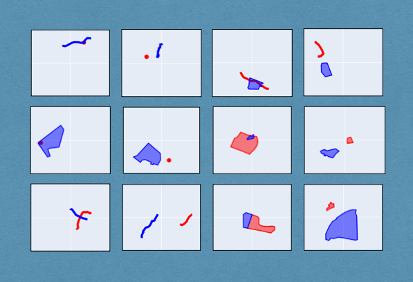
Pictures say more than words, so here are some cases from the synthetic dataset.
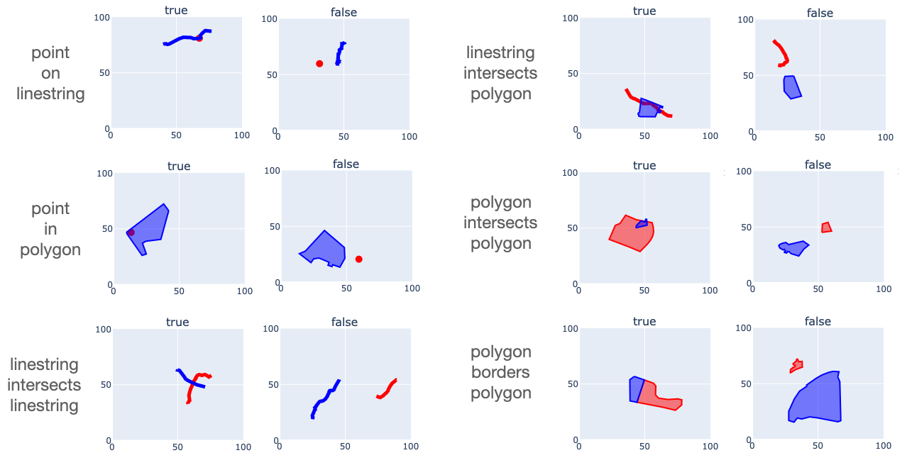
Overall, I generated 20,000 true cases and 20,000 false cases for each of the six relations shown above. That gfives us material for training models.
Predicting relations from encodings
To check whether MPP encodings can capture spatial relationships, we can try training a model whose input is a pair of encodings, and whose output is a prediction of whether a given relation holds. That is, a model is trained to answer a question like "do these two lines intersect?" or "does this point lie inside this polygon?" If such model performs well, it proves that the encodings capture the relation.
In the example that I will give below, all models are neural networks with similar structure. The input is a concatenation $\mathbf{e}(\mathbf{a}_i) || \mathbf{e}(\mathbf{b}_i)$ of the encodings of a pair of geometries $\mathbf{a}_i$ and $\mathbf{b}_i$. The models have two fully connected linear layers of size 128, and an output layer that produces a single value. The final layer uses a sigmoid activation function, so the output is between 0 and 1, allowing the model to be trained with a binary cross entropy loss function.
One can evaluate such model using the ROC AUC metric, which is essentially the probability that the model will rate a true case higher than a false case.
To train a model, we take the synthetic data giving the true and false cases for a relation, and use 60% for training, 20% for validation (to determine when to stop training) and 20% for final model testing. All performance numbers below are the respective model's ROC AUC for the test set.
Comparisons
My previous post discussing position encodings compared Multi-Point Proximity (MPP) encoding with a simpler method based on Discrete Indicator Vectors (DIV) for tiles covering the region of interest. We will continue comparing those two methods in this analysis. That is, all models were trained first using DIV-encoded shapes, and then using MPP-encoded shapes.
The previous post also suggested that a key consideration for such encodings is their resolution, and that one might expect better performance using finer resolution. For MPP encodings, the resolution is the spacing between the reference points. For DIV encoding it is the size of the tiles used to cover the region of interest. There is a direct correspondence between the resolution values of the two methods: an MPP reference point spacing of $x$ produces encodings of the same size as a DIV encoding with tile size $x$.
I trained all models on encodings with resolutions of 50, 33.3, 25, 20, 10, 6.25, and 5. Those number correspond to grids of size $2\times2$, $3\times3$, $4\times4$, $5\times5$, $10\times10$, $16\times16$, and $20\times20$ within the $100\times100$ region of interest.
This is what the results look like.
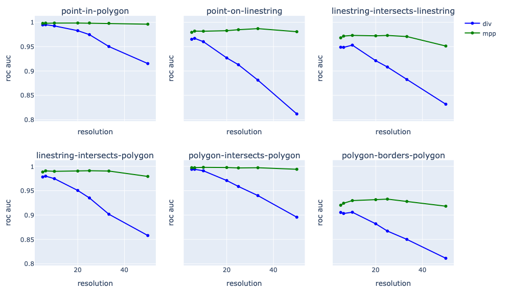
Some clear trends are:
- ROC AUC values are consistently high, indicating that the encodings capture spatial relations well. Performance varies by relation type, which suggests that some are harder to capture than others. The only case with values lower than 0.95 is the "polygon-borders-polygon" relation. That's a fairly difficult case to get right, since two polygons that have a very slight separation or a very small overlap don't "border" one another, so they would be false cases that look a lot like true cases. Still the performance is quite good overall.
- MPP encodings consistently yield better performance than DIV encodings. This is mostly expected based on discussions in the previous post, and has been suggested to be the case in the literature [6].
- There is a decline in performance as we move to coarser resolutions. This too is hardly a surprise: finer resolutions always capture more detail. But a clear trend is that MPP encodings are less affected by degraded resolution than DIV approaches. So one might be able to get away with coarser resolution / smaller data volumes / less processing without significant degradation of performance for some applications.
- There is one strange trend in that the finest resolutions sometimes yield decreased performance relative to moderate ones. I don't yet have an explanation, but it may be due to the increase in the size of the model for these cases. Finer resolution means more trainable weights, which could cause difficulty training and may require a larger dataset to yield the same performance levels. But that remains to be confirmed.
Discussion
This analysis has shown that shape encodings capture information about pairwise geospatial relationships between objects. The performance is not 100%, since the encodings are approximations. But the trade-off with performance is the ability to use shapes with ML and AI models. And that opens the door to at least three very promising types of applications.
First, MPP encodings could serve a purpose analogous to positional encodings in text processing. Large Language Models (LLMs) require word order to be expressed explicitly because transformer processing is not sufficiently sensitive to the ordering of its inputs. That requirement has led to the use of widely known methods like sinusoidal position encoding [5] and rotary position encoding [4]. There is a need for an analogous encoding scheme for spatial AI and ML models – something that applies to any shape, and that captures information about the properties of the shape itself and its relationship to other shapes in a region. This series of blog posts has shown that the MPP method possesses exactly those characteristics.
Second, spatial encodings can serve as a component of a Spatial Representation Learning (SRL) pipeline, providing the initial "vectorization" of geometric shapes for input to a Neural Network model that learns deep embeddings. This has been recognized as a key technology that will enable the next generation of geospatial AI [3].
Third, spatial encodings can be used as an index in vector databases. Such databases are a critical component of Retrieval Augmented Generation (RAG), which has proven so powerful in AI applications. Any element in the database is indexed by a vector, and query results are based on their similarity to a query vector. In text-based RAG, the query vector is typically an embedding of a question asked in natural language, and the query yields relevant passages from source documents to serve as context for a LLM-generated response. The analogy in geospatial processing would be where one seeks information associated with a geographical entity – a region, a roadway, a river, etc. – from a database of other geographical entities that are indexed by their encodings. The encoding of the "query shape" could be used to retrieve information about objects that are spatially similar, in the sense of being in the same general vicinity and having a similar form.
Conclusion
I hope that my series of posts on this topic has convinced you of the potential of geospatial encodings, and has given you some ideas about how these methods can be used to further develop the field of Geospatial AI. If so, I would love to hear about them. Get a discussion going in the comments!
Revision History
- April 11, 2025: Initial release
- April 17, 2025: Removed a heading for an empty section.
References
[1]: Gengchen Mai, Krzysztof Janowicz, Yingjie Hu, Song Gao, Bo Yan, Rui Zhu, Ling Cai, and Ni Lao, A review of location encoding for GeoAI: methods and applications, International Journal of Geographical Information Science, Volume 36(4), Jan 2022.
[2]: Gengchen Mai, Yiqun Xie, Xiaowei Jia, Ni Lao, Jinmeng Rao, Qing Zhu, Zeping Liu, Yao-Yi Chiang, Junfeng Jiao, Towards the next generation of Geospatial Artificial Intelligence, International Journal of Applied Earth Observation and Geoinformation, Volume 136, 2025, 104368, ISSN 1569-8432.
[3]: Gengchen Mai, Xiaobai Yao, Yiqun Xie, Jinmeng Rao, Hao Li, Qing Zhu, Ziyuan Li, and Ni Lao. 2024. SRL: Towards a General-Purpose Framework for Spatial Representation Learning. In Proceedings of the 32nd ACM International Conference on Advances in Geographic Information Systems (SIGSPATIAL '24). Association for Computing Machinery, New York, NY, USA, 465–468.
[4]: Jianlin Su and Yu Lu and Shengfeng Pan and Ahmed Murtadha and Bo Wen and Yunfeng Liu. 2023. RoFormer: Enhanced Transformer with Rotary Position Embedding}, arXiv: https://arxiv.org/abs/2104.09864.
[5] Ashish Vaswani, Noam Shazeer, Niki Parmar, Jakob Uszkoreit, Llion Jones, Aidan N. Gomez, Łukasz Kaiser, and Illia Polosukhin. 2017. Attention is all you need. In Proceedings of the 31st International Conference on Neural Information Processing Systems (NIPS'17). Curran Associates Inc., Red Hook, NY, USA, 6000–6010.
[6]: Yin, Y., et al., 2019. GPS2Vec: Towards generating worldwide GPS embeddings. In: ACM SIGSPATIAL 2019. 416–419.
[7] G. Boeing, 2024. Modeling and Analyzing Urban Networks and Amenities with OSMnx. Working paper.
Comments ()